Lab 9: Interactions between continuous variables

PSYC 7804 - Regression with Lab

Fabio Setti

Spring 2025

Today’s Packages and Data 🤗

Install Packages Code

# devtools::install_github("quinix45/FabioFun")
install.packages("interactions")

library(tidyverse)
library(interactions)
library(FabioFun)
theme_set(theme_classic(base_size = 14, 
                        base_family = 'serif'))

interactions

The interactions package (Long, 2024) provides helpful functions to explore interaction effects.

Data

dat <- rio::import("https://github.com/quinix45/PSYC-7804-Regression-Lab-Slides/raw/refs/heads/main/Slides%20Files/Data/Attend.dta")

# select only the variables we are interested in
grade_fin <- dat[,c("final", "attend", "priGPA")]

Why Interactions?

The idea of interaction is that the effect two predictors \(X_1\) and \(X_2\) have on an outcome \(Y\) is fundamentally tied together.

More specifically, the effect that \(X_1\) has on \(Y\) depends on the value of \(X_2\), and the effect that \(X_2\) has on \(Y\) depends on the value of \(X_1\).

A very clear example of an interaction effect is how an individual’s gender and race jointly affect number of experienced daily microagressions. Looking at gender and race separately would miss much of the picture (intersectionality!)

If we believe that two variables should interact in how they influence \(Y\), we can express that with the regression model:

\[ \hat{Y} = b_0 + b_1X_1 + b_2X_2 + b_3(X_1 \times X_2) \]

By the way, Interaction or Moderation?

Interaction and moderation are the same exact thing.

I prefer the term interaction to avoid confusion with the term mediation, which has absolutely nothing to do with anything discussed in this Lab. That being said …

When hypothesizing interaction effects, it is useful to make a distinction between a focal predictor and a moderator.

Interactions are usually represented with the diagrams on the right. the variable pointing directly to \(Y\) is considered the focal predictor, while the variable pointing to the line is considered the moderator.

The two representation on the right are equivalent. However, depending on your hypotheses it may make more practical sense to conceptualize one variables as the focal predictor and the other as the moderator.

Our hypothesis

We hypothesize that the grade on a statistics final (final, \(Y\)) is predicted by how many classes a student attends (attend, \(X_1\)). Additionally, we also think that the effect that attend has on final is moderated by prior GPA before starting the class (priGPA, \(X_2\)).

# we use "*" to specify an interaction effect between two variables
reg_int <- lm(final ~ attend*priGPA, data = grade_fin)
summary(reg_int)


Call:
lm(formula = final ~ attend * priGPA, data = grade_fin)

Residuals:
     Min       1Q   Median       3Q      Max 
-16.4387  -2.8093  -0.2672   3.0143  11.3030 

Coefficients:
              Estimate Std. Error t value Pr(>|t|)    
(Intercept)   30.14293    3.66576   8.223 1.02e-15 ***
attend        -0.47663    0.13773  -3.461 0.000573 ***
priGPA        -2.21470    1.62020  -1.367 0.172101    
attend:priGPA  0.20231    0.05878   3.441 0.000614 ***
---
Signif. codes:  0 '***' 0.001 '**' 0.01 '*' 0.05 '.' 0.1 ' ' 1

Residual standard error: 4.354 on 676 degrees of freedom
Multiple R-squared:  0.1491,    Adjusted R-squared:  0.1454 
F-statistic:  39.5 on 3 and 676 DF,  p-value: < 2.2e-16

our regression equation is:

\[ \hat{Y} = 30. 14 - 0.48X_1 - 2.21X_2 + 0.20 X_1 X_2 \]

Crucially, our interaction term is significantly different from 0. The intercept, \(30.14\), is still the expected value of \(Y\) when \(X_1 = 0\) and \(X_2 = 0\)…

However, now that we are dealing with a significant interaction effect, \(0.20 X_1 X_2\), things are not so simple! The slopes now have very specific meanings 🧐

Visualizing Interactions

We can visualize what interaction effects imply graphically. Interactions between continuous variables bend the regression plane:

Plot Code

library(plotly)

FabioFun::nice_3D_plot(y = grade_fin$final,
                       x1 = grade_fin$priGPA,
                       x2 = grade_fin$attend,
                       axis_names = c("Final",
                                      "Prior GPA",
                                      "Attendance"),
                       reg_plane = TRUE,
             opacity = 0.3) %>% 
   layout(title = 'Regression Plane with no Interaction')%>%  
  bslib::card(full_screen = TRUE)

Plot Code

FabioFun::nice_3D_plot(y = grade_fin$final,
                       x1 = grade_fin$priGPA,
                       x2 = grade_fin$attend,
                       axis_names = c("Final",
                                      "Prior GPA",
                                      "Attendance"),
                       reg_plane = TRUE, 
                       interaction = TRUE,
             opacity = 0.3)%>% 
  layout(title = 'Regression Plane with Interaction')%>%  
  bslib::card(full_screen = TRUE)

Regression Planes Bend?

So what does it mean for a regression plane to bend or not? We can start by thinking about the regression equation without any interactions.

if we say:

\[ \hat{Y} = b_0 + b_1X_1 + b_2X_2 \] You can see that the slopes of \(b_1\) and \(b_2\) are always constant, no matter what values you plug in the equation.

This means that we believe that the relation that \(X_1\) and \(X_2\) have on \(Y\) is independent.

A regression plane is flat on the surface only when the slopes are always constant (i.e. no interaction is assumed).

Plot Code

FabioFun::nice_3D_plot(y = grade_fin$final,
                       x1 = grade_fin$priGPA,
                       x2 = grade_fin$attend,
                       axis_names = c("Final",
                                      "Prior GPA",
                                      "Attendance"),
                       reg_plane = TRUE,
             opacity = 0.3) %>% 
   layout(title = 'Regression Plane with no Interaction')%>%  
  bslib::card(full_screen = TRUE)

Regression Planes Bend Indeed!

Instead, if we say:

\[ \hat{Y} = b_0 + b_1X_1 + b_2X_2 + b_3X_1 X_2 \] You can see that the slopes of \(X_1\) and \(X_2\) will respectively change depending on what values you give to \(X_1\) or \(X_2\). Let’s say that \(X_2 = 2\). Then:

\(\hat{Y} = b_0 + b_1X_1 + 2b_2 + 2b_3X_1\)

↓

\(\hat{Y} = (b_0 + 2b_2) + (b_1 + 2b_3)X_1\)

If a slope is the relation between \(X\) and \(Y\), an interaction implies that the relation changes depending on the value of another variable. This is represented by the plane bending, reflecting the change in slope.

Plot Code

FabioFun::nice_3D_plot(y = grade_fin$final,
                       x1 = grade_fin$priGPA,
                       x2 = grade_fin$attend,
                       axis_names = c("Final",
                                      "Prior GPA",
                                      "Attendance"),
                       reg_plane = TRUE,
                       interaction = TRUE,
             opacity = 0.3) %>% 
   layout(title = 'Regression Plane with no Interaction') %>%  
  bslib::card(full_screen = TRUE)

What about the Regression coefficients?

With that in mind, our variables were final grade (\(Y\)), attendance (\(X_1\)), and GPA prior to taking the class (\(X_2\)):

\[ \hat{Y} = 30. 14 - 0.48X_1 - 2.21X_2 + 0.20 X_1 X_2 \]

If you look at the regression coefficients for \(X_1\) and \(X_2\), you will see that they are negative, meaning that…as GPA prior to taking the class and attendance increase, the final grade…decreases?!🤨

The regression coefficients of \(X_1\) and \(X_2\) shown here are the slopes on the plane, when either \(X_1 = 0\) or \(X_2 = 0\). The minimum value of our predictors is respectively:

min(grade_fin$attend)

[1] 2

min(grade_fin$priGPA)

[1] 0.857

So we are looking at the slopes at a single point of the plane that does not have any data…that’s not very useful 😧

This is also why you do not interpret slopes individually with a significant interaction effect. They only capture a small fraction of the regression plane.

Still, we can pull some shenanigans to make the meaning of \(X_1 = 0\) or \(X_2 = 0\) more informative 😀 Any ideas?

Mean Centering

Turns out that we can transform our variables such that we can decide the meaning of \(0\)! Transforming our dependent variables such that \(0\) represents the mean is generally a good choice.

We can use the scale() function to center our predictors:

# the scale() function is a bit strange as previously mentioned, so we need to add the [,1] (see what happens to the column name if you don't)
# `scale = FALSE` tells the fucntion to not standardize the variable (i.e., do not make the standard deviation 1)

grade_fin$attend_cnt <- scale(grade_fin$attend, scale = FALSE)[,1]
grade_fin$priGPA_cnt <- scale(grade_fin$priGPA, scale = FALSE)[,1]

Centering changes the means of the variables to 0, but does not change the standard deviations:

Mean (row 1) and SD (row 2) of uncentered variables

round(rbind(apply(grade_fin[, 2:3], 2, mean),
            apply(grade_fin[, 2:3], 2, sd)), 2)

     attend priGPA
[1,]  26.15   2.59
[2,]   5.46   0.54

Mean (row 1) and SD (row 2) of centered variables

round(rbind(apply(grade_fin[, 4:5], 2, mean),
            apply(grade_fin[, 4:5], 2, sd)), 2)

     attend_cnt priGPA_cnt
[1,]       0.00       0.00
[2,]       5.46       0.54

Mean Centering Graphically

Changing the mean of a variable simply means shifting it along the x-axis. For example, if we plot the density of the uncentered and centered attend variable:

Plot Code

grade_fin %>% 
  ggplot(aes(x = attend)) +
  geom_density(col = "red") +
  geom_density(aes(x = attend_cnt), col = "blue") +
  xlim(-30, 40) +
  xlab("Centerd and Uncentered Distribution of `attend`")

The red distribution is the original uncentered variable.
the blue distribution is the mean centered variable.

Linear Transformations

Centering and standardizing are known as linear transformations. The “linear” comes from the fact that all these transformations do is shift all the data along a line. You can see that from the graph on the left. These transformations have no effect on the results of statistical analyses, but can make interpretation easier.

Uncentered and Centered Results

#uncentered
reg_int <- lm(final ~ attend*priGPA, data = grade_fin)
summary(reg_int)


Call:
lm(formula = final ~ attend * priGPA, data = grade_fin)

Residuals:
     Min       1Q   Median       3Q      Max 
-16.4387  -2.8093  -0.2672   3.0143  11.3030 

Coefficients:
              Estimate Std. Error t value Pr(>|t|)    
(Intercept)   30.14293    3.66576   8.223 1.02e-15 ***
attend        -0.47663    0.13773  -3.461 0.000573 ***
priGPA        -2.21470    1.62020  -1.367 0.172101    
attend:priGPA  0.20231    0.05878   3.441 0.000614 ***
---
Signif. codes:  0 '***' 0.001 '**' 0.01 '*' 0.05 '.' 0.1 ' ' 1

Residual standard error: 4.354 on 676 degrees of freedom
Multiple R-squared:  0.1491,    Adjusted R-squared:  0.1454 
F-statistic:  39.5 on 3 and 676 DF,  p-value: < 2.2e-16

# centered
reg_int_cnt <- lm(final ~ attend_cnt*priGPA_cnt, data = grade_fin)
summary(reg_int_cnt)


Call:
lm(formula = final ~ attend_cnt * priGPA_cnt, data = grade_fin)

Residuals:
     Min       1Q   Median       3Q      Max 
-16.4387  -2.8093  -0.2672   3.0143  11.3030 

Coefficients:
                      Estimate Std. Error t value Pr(>|t|)    
(Intercept)           25.63475    0.18284 140.202  < 2e-16 ***
attend_cnt             0.04669    0.03863   1.209 0.227255    
priGPA_cnt             3.07500    0.34254   8.977  < 2e-16 ***
attend_cnt:priGPA_cnt  0.20231    0.05878   3.441 0.000614 ***
---
Signif. codes:  0 '***' 0.001 '**' 0.01 '*' 0.05 '.' 0.1 ' ' 1

Residual standard error: 4.354 on 676 degrees of freedom
Multiple R-squared:  0.1491,    Adjusted R-squared:  0.1454 
F-statistic:  39.5 on 3 and 676 DF,  p-value: < 2.2e-16

What Changed?

We can see that the value of the interaction term remains the same, but the values of the intercept and the slopes for \(X_1\) and \(X_2\) change:

Uncentered Result

\[ \hat{Y} = 30. 14 - 0.48X_1 - 2.21X_2 + 0.20 X_1 X_2 \]

Centered Result

\[ \hat{Y} = 25. 63 + 0.47X_1 + 3.08X_2 + 0.20 X_1 X_2 \]

In the centered result, where \(0\) represents the mean of \(X_1\) and \(X_2\), both slopes are positive, and indicate that as GPA prior to taking the class and as attendance increases, the final grade…increases!

Nothing changed about our analysis, but in the centered solution, we are looking at the slopes at a different point of the regression plane. This point is not out of range, so it makes sense to choose it as a reference point.

Regression Coefficients Flipping When Centering? 🤔

The regression coefficients flipping signs is reflected by the direction of the plane flipping. Look for that on the plot on the next slide. You should see that the plane changes direction as some point as the values of the predictors change.

Graphical comparison

The plane and the data in the centered version on the right has been shifted such that the \(0\) point for both predictors corresponds to a location where we have most of our data. On the left, there is no data at the \(0\) point for either predictors.

Plot Code

FabioFun::nice_3D_plot(y = grade_fin$final,
                       x1 = grade_fin$priGPA,
                       x2 = grade_fin$attend,
                       axis_names = c("Final",
                                      "Prior GPA",
                                      "Attendance"),
                       reg_plane = TRUE, 
                       interaction = TRUE,
             opacity = 0.2)%>% 
  layout(title = 'Uncentered')%>%  
  bslib::card(full_screen = TRUE)

Plot Code

FabioFun::nice_3D_plot(y = grade_fin$final,
                       x1 = grade_fin$priGPA_cnt,
                       x2 = grade_fin$attend_cnt,
                       axis_names = c("Final",
                                      "Prior GPA",
                                      "Attendance"),
                       reg_plane = TRUE, 
                       interaction = TRUE,
             opacity = 0.2)%>% 
  layout(title = 'Centered')%>%  
  bslib::card(full_screen = TRUE)

The Interpretation of The Interaction Term

So far we have discussed why we should not interpret slopes in isolation, but what does the interaction effect, \(0.20\), mean in our case?

\(0.20\) is the expected change in slope of one predictor per 1-unit change in the other predictor.

so, if our equation is \(\hat{Y} = 25. 63 + 0.47X_1 + 3.08X_2 + 0.20 X_1 X_2\)

For a prior GPA of \(X_2 = 3.5\) we get:

\(\hat{Y} = 25.63 + 0.47X_1 + 3.08 \times 3.5 + 0.20 X_1\times 3.5\)

\(\hat{Y} = (25.63 + 10.78) + 0.47X_1 + 0.7X_1\)

\(\hat{Y} = 36.41 + 1.17X_1\)

NOTE: If you paid attention, now that \(X_2\) is centered, \(3.5\) does not actually mean a GPA of \(3.5\). Here, for the sake of the interpretation and plugging in some numbers, I assume it means a GPA of \(3.5\), although that is incorrect.

So, when someone starts the class with a prior GPA of \(3.5\), the relation between attendance and final grade strengthens: the slope of \(X_1\) goes from \(0.47\) to \(1.17\).

Sounds Familiar?

If you remember, the interpretation of the quadratic term in Lab 8 is suspiciously similar to an interaction effect 🧐 Could it be that the quadratic term is also an interaction effect? Give it some thought 🤔

Probing Interactions: Simple Slopes

On the previous slide, we plugged in some value for \(X_2\) and looked at the resulting value of the slope for \(X_1\). The resulting \(1.17\) value for the slope of \(X_1\) is generally referred to as a simple slope.

When testing specific hypotheses, you plug in values for your moderator variable, and look the resulting slopes of the focal predictor. Generally, we choose to look at the simple slopes of the focal predictor at the mean of the moderator and at 1 SD below/above the mean of the moderator.

# you need to specify which variable is the focal predictor (`pred =`) and which is the moderator (`modx =`)!

sim_slopes <- interactions::sim_slopes(reg_int_cnt, 
                                       modx = "priGPA_cnt",
                                       pred = "attend_cnt")

# rounding to 3 decimal places for nicer output
round(sim_slopes$slopes,3)

  Value of priGPA_cnt   Est.  S.E.   2.5% 97.5% t val.     p
1              -0.545 -0.064 0.036 -0.135 0.008 -1.742 0.082
2               0.000  0.047 0.039 -0.029 0.123  1.209 0.227
3               0.545  0.157 0.061  0.037 0.276  2.577 0.010

The simple slopes are under the Est. column. Any questions about the other columns?

Notice that only once priGPA is 1 SD above the mean is the slope of attend_cnt positive and significant. That suggests that attendance helps with the final grade only if you prior GPA is 1 SD above average.

Practical implication? Only students who are already good benefit from going to class. The teacher in this class is not the best 😱

Plotting Simple Slopes

The code below plots the simple slopes at different values of the moderator:

interact_plot(reg_int_cnt, 
              modx = "priGPA_cnt",
              pred = "attend_cnt")

You can also think of the slopes in this plot as a snapshot of the direction of the regression plane at a specific value of the moderator!

Plotting Simple Slopes

We can also specify values of the moderator manually:

interact_plot(reg_int_cnt, 
     modx = "priGPA_cnt",
     pred = "attend_cnt",
     modx.values = c(-4, 3, 4))

The johnson-neyman Plot 😱

Instead the simple slopes, we can visualize how the slope of the focal predictor changes as the moderator changes:

johnson_neyman(reg_int_cnt, 
              modx = "priGPA_cnt",
              pred = "attend_cnt")

x-axis: the value of the moderator.
y-axis: the value of the slope of the focal predictor (make sure this makes sense to you!)

The blue band means that the slope of the focal predictor is significant at the value of the moderator.

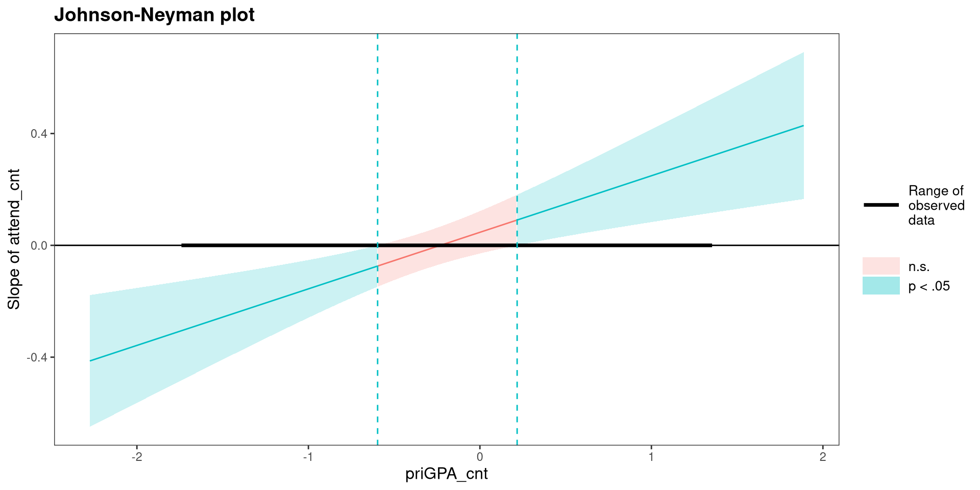
Advice: If you are presenting your research and interactions are involved…I would use simple slopes instead of a Johnson-Neyman plot. Why? It’s an absolute truth about the universe that Johnson-Neyman plots are confusing 🤷 keep it simple.

References

Becker, J., Chan, C., Schoch, D., Chan, G. C., Leeper, T. J., Gandrud, C., MacDonald, A., Zahn, I., Stadlmann, S., Williamson, R., Kennedy, P., Price, R., Davis, T. L., Day, N., Denney, B., Bokov, A., & Gruson, H. (2024). Rio: A Swiss-Army Knife for Data I/O (Version 1.2.3) [Computer software]. https://cran.r-project.org/web/packages/rio/index.html

Long, J. A. (2024). Interactions: Comprehensive, User-Friendly Toolkit for Probing Interactions (Version 1.2.0) [Computer software]. https://cran.r-project.org/web/packages/interactions/index.html

Wickham, H., & RStudio. (2023). Tidyverse: Easily Install and Load the ’Tidyverse’ (Version 2.0.0) [Computer software]. https://cran.r-project.org/web/packages/tidyverse/index.html